Chern Simons Theory and Yang-Baxter Equation

Nov 18, 2025 · updated May 22, 2026

Chern-Simons Theory

Chern-Simons theory is a topological version of Yang-Mills theory defined on a three-dimensional manifold $𝑋$ . In this case, the gauge connection $𝐴$ takes values in the Lie algebra $𝔤$ of the gauge group $𝐺$ , and the Chern-Simons action is given by:

{CS}_{𝑋} [𝐴] = \int_{𝑋} tr (𝐴 𝑑 𝐴 + \frac{2}{3} 𝐴^{3}),

where $𝐴$ is a connection 1-form on a principal $𝐺$ -bundle over $𝑋$ . In physical literature, people often consider the Chern-Simons action with a coupling constant $𝑘$ :

𝑆_{CS}^{𝑘} [𝐴] = \frac{𝑘}{4 𝜋} {CS}_{𝑋} [𝐴] .

where $𝑘$ is quantized to ensure gauge invariance at the quantum level. Formally, using the path integral formalism, the partition function of Chern-Simons theory is formally given by:

𝑍_{CS}^{𝑘} (𝑋) = \int 𝑑 𝜇_{𝑋} [𝐴] 𝑒^{𝑖 𝑆_{CS}^{𝑘} [𝐴]},

i.e., integrating over the quotient space of the space of all connections in $𝐺$ -bundles over $𝑋$ modulo gauge transformations.

At the perturbative level, the partition function is expanded around flat connections $𝐴_{0}$ satisfying $𝐹_{𝐴_{0}} = 0$ , which is the classical equation of motion derived from the Chern-Simons action.

Wilson Loops

The gauge-invariant observables in Chern-Simons theory are Wilson loops, which are defined with data $(𝐾, 𝜌)$ , where $𝐾 : 𝕊^{1} ↪︎ 𝑋$ is a knot embedded in $𝑋$ , and $𝜌 : 𝐺 \to GL (𝑉)$ is a representation of the gauge group $𝐺$ on a vector space $𝑉$ , and could be written as:

𝑊_{𝐾} (𝜌) = {tr}_{𝜌} 𝒫︀ exp (\int_{𝐾} 𝑖 𝐴),

where $𝒫︀ exp$ denotes the path-ordered exponential along the knot $𝐾$ .

In our previous blog about anyons, such Wilson loop observable can be interpreted as the world line of a particle moving in $𝑋$ and carrying some charge under the gauge group $𝐺$ . Where the charge of this particle is labeled by the representation $𝜌$ .

Remark

Physically speaking, the Wilson loop can be interpreted as following:

$𝐾$ in a generic position (a Morse knot) $\Leftrightarrow$ world line of a particle moving in $𝑋$ .
$𝜌$ $\Leftrightarrow$ charge of this particle under the gauge group $𝐺$ .

Where Morse knot means the height function (w.r.t. some fixed direction, which is the time direction in a physical context) restricted to the knot is a Morse function.

Remark

Physically speaking, the Wilson loop can be interpreted as following:

$𝐾$ in a generic position (a Morse knot) $\Leftrightarrow$ world line of a particle moving in $𝑋$ .
$𝜌$ $\Leftrightarrow$ charge of this particle under the gauge group $𝐺$ .

Where Morse knot means the height function (w.r.t. some fixed direction, which is the time direction in a physical context) restricted to the knot is a Morse function.

The quantum expectation value of a Wilson loop could be formally defined as:

⟨ 𝑊_{𝐾_{1}} (𝜌_{1}) \dots 𝑊_{𝐾_{𝑛}} (𝜌_{𝑛}) ⟩ = \frac{1}{𝑍_{CS} (𝑋)} \int 𝑑 𝜇_{𝑋} [𝐴] 𝑒^{𝑖 𝑆_{CS} [𝐴]} 𝑊_{𝐾_{1}} (𝜌_{1}) \dots 𝑊_{𝐾_{𝑛}} (𝜌_{𝑛}) .

Remarkably, due to the work of Witten, these expectation values yield topological invariants (Jones polynomial) of the knots and links in $𝑋 = 𝕊^{3}$ .

Witten’s approach uses non-perturbative methods, relating Chern-Simons theory to conformal field theory (Wess-Zumino-Witten theory) on the boundary of $𝑋$ , and employing surgery techniques to compute these invariants.

A natural question is: can we recover these knot invariants using perturbative methods? At this level, a natural expectation is, the result would (at least formally) correspond to the Taylor coefficients of some knot polynomial invariants, and each coefficient could be a new knot invariant. In this blog, we would see that this is indeed the case.

Kontsevich Integral from Chern-Simons Theory

From now on, we assume $𝑋 = ℝ \times Σ$ , where $Σ$ is a Riemann surface and $ℝ$ denotes the time direction. In this case, the Morse knots could be defined with respect to the height function along the $ℝ$ direction.

We also choose a set of bases ${𝑡_{𝑎}}$ for gauge Lie algebra $𝔤$ , such that $tr (𝑡_{𝑎} 𝑡_{𝑏}) = 𝛿_{𝑎 𝑏}$ , $[𝑡_{𝑖}, 𝑡_{𝑗}] = 𝑓_{𝑖 𝑗}^{𝑘} 𝑡_{𝑘}$ . Then the gauge connection $𝐴$ could be expressed as $𝐴 = 𝐴^{𝑎} 𝑡_{𝑎}$ , where $𝐴^{𝑎} \in Ω^{1} (𝑋)$ are ordinary 1-forms on $𝑋$ (after choosing a reference trivialization of the principal $𝐺$ -bundle).

To perform perturbative expansion, we need to fix a gauge. In this case, a natural gauge fixing condition could be realized following. First, given a complex structure on $Σ$ , we could introduce complex coordinates $(𝑧, 𝑧)$ on $Σ$ . Then the gauge connection $𝐴$ could be decomposed as:

𝐴 (𝑧, 𝑧, 𝑡) = 𝐴_{𝑡} 𝑑 𝑡 + 𝐴_{𝑧} 𝑑 𝑧 + 𝐴_{𝑧} 𝑑 𝑧 .

We shall impose the axial gauge condition (a.k.a holomorphic gauge) $𝐴_{𝑧} = 0$ . Thus, the gauge connection reduces to $𝐴 (𝑧, 𝑡) = 𝐴_{0} 𝑑 𝑡 + 𝐴_{𝑧} 𝑑 𝑧$ , and the Chern-Simons action simplifies to:

{CS}_{𝑋} [𝐴] ≔ \int_{𝑋} 𝐴 𝜕_{𝑡} 𝐴,

where $𝜕_{𝑡} ≔ 𝑑 𝑡 𝜕$ . Under this gauge fixing, the path integral would be reduced to a purely Gaussian integral.

To using the perturbative method, we need to compute the propagator (two-point correlation function) of the gauge field $𝐴$ . At the axial gauge, the propagator could be computed as:

⟨ 𝐴_{𝑖}^{𝑎} (𝑧_{1}, 𝑡_{1}) 𝐴_{𝑗}^{𝑏} (𝑧_{2}, 𝑡_{2}) ⟩ = 𝛿^{𝑎 𝑏} \frac{1}{𝑖 𝑘} \frac{𝑑 𝑧_{1} - 𝑑 𝑧_{2}}{𝑧_{1} - 𝑧_{2}} 𝛿 (𝑡_{1} - 𝑡_{2}) .

Thus, the expectation value of Wilson loops could be computed using Wick’s theorem. To compute this expectation value, we choose a Morse knot $𝐾$ embedded in $𝑋$ and a parameterization $𝛾 : [0, 1] ↪︎ 𝐾 \subset 𝑋$ of the knot. Then the Wilson loop observable could be expanded as:

𝑊_{𝐾} (𝜌) = 1 + \sum_{𝑛 = 1}^{\infty} 𝑖^{𝑛} {tr}_{𝜌} \int_{0 \leq 𝑡_{1} \leq \dots \leq 𝑡_{𝑛} \leq 1} 𝐴 (𝛾 (𝑡_{1})) \dots 𝐴 (𝛾 (𝑡_{𝑛})),

using the decomposition of the gauge field $𝐴 = 𝐴^{𝑎} 𝑡_{𝑎}$ , we could rewrite this as:

𝑊_{𝐾} (𝜌) = 1 + \sum_{𝑛 = 1}^{\infty} 𝑖^{𝑛} \sum_{𝑎_{1}, \dots, 𝑎_{𝑛}} {tr}_{𝜌} (𝑡_{𝑎_{1}} \dots 𝑡_{𝑎_{𝑛}}) \int_{0 \leq 𝑡_{1} \leq \dots \leq 𝑡_{𝑛} \leq 1} 𝐴^{𝑎_{1}} (𝛾 (𝑡_{1})) \dots 𝐴^{𝑎_{𝑛}} (𝛾 (𝑡_{𝑛})) .

Thus, the expectation value could be computed with:

⟨ 𝐴^{𝑎_{1}} (𝑧 (𝑡_{1}), 𝑡_{1}) \dots 𝐴^{𝑎_{2 𝑛}} (𝑧 (𝑡_{2 𝑛}), 𝑡_{2 𝑛}) ⟩ = {(\frac{1}{𝑖 𝑘})}^{𝑛} {tr}_{𝜌} \sum_{𝑃} {(- 1)}^{# ↓ 𝑃} \underset{𝑙 \in 𝑃}{⋀} \frac{𝑑 𝑧_{𝑙_{1}} - 𝑑 𝑧_{𝑙_{2}}}{𝑧_{𝑙_{1}} - 𝑧_{𝑙_{2}}} 𝛿 (𝑡_{𝑙_{1}} - 𝑡_{𝑙_{2}}),

where $𝑃$ is a pairing of the set ${1, \dots, 2 𝑛}$ , each pair $𝑙 \in 𝑃$ consists of two elements $(𝑙_{1}, 𝑙_{2})$ , and $# ↓ 𝑃$ denotes the number of arcs that are oriented downwards when equipped with the inherited orientation from $𝐾$ .

After integrating out the delta functions, the linked vertex would live at a same time slice along the $ℝ$ direction. Thus, the expectation value of the Wilson loop could be expressed as:

⟨ 𝑊_{𝐾} (𝜌) ⟩ = \sum_{𝑛 = 0}^{\infty} \frac{1}{𝑘^{𝑛}} {tr}_{𝜌} Φ_{𝑛} (𝐾),

where $Φ_{𝑛} (𝐾)$ is called the Kontsevich integral of the knot $𝐾$ , which could be expressed as:

Φ_{𝑛} (𝐾) = \sum_{𝑃} \underset{𝑙 \in 𝑃}{⋀} {(- 1)}^{# ↓ 𝑃} \int_{0 \leq 𝑡_{1} \leq \dots \leq 𝑡_{𝑛} \leq 1} \frac{𝑑 𝑧_{𝑙_{1}} - 𝑑 𝑧_{𝑙_{2}}}{𝑧_{𝑙_{1}} - 𝑧_{𝑙_{2}}} Ω_{𝑙} .

where $Ω_{𝑙} = 𝜌 (𝑡_{𝑙_{1}}) \otimes 𝜌 (𝑡_{𝑙_{2}})$ is an double insertion of Lie algebra elements at the points $𝛾 (𝑡_{𝑙_{1}})$ and $𝛾 (𝑡_{𝑙_{2}})$ on the knot, which could be read from “linking” the knot at these two points with weight $Ω_{𝑙}$ .

It is not hard to see that, the definition of $Φ_{𝑛} (𝐾)$ is (the non-abelian generalization of) the time evolution operator we constructed in the anyon system discussed in previous blog. So, you may think that the Kontsevich integral could be interpreted as the time evolution operator of some anyon system moving along the world line $𝐾$ in the presence of statistics interaction.

Remark

Well, there is an additional factor ${(- 1)}^{# ↓ 𝑃}$ in the definition of $Φ_{𝑛} (𝐾)$ , which is absent in the anyon system. This is because, in the anyon system, the height function should have no critical points along the world line, thus, such factor is always trivial. Thus, in this sense, Chern-Simons theory includes the “anti-anyon” effect naturally, which is absent in the simple anyon system we constructed above.

An interesting question is, could we construct some anyon system that includes such “anti-anyon” effect?

Remark

An interesting question is, could we construct some anyon system that includes such “anti-anyon” effect?

Example: R-matrix from Kontsevich Integral

We consider a simple braiding configuration of two strands, which is a simple Morse knot embedded in $ℝ \times ℂ$ .

The intersection of two strands at a time slice would become two distinct points $𝑧_{1}, 𝑧_{2}$ in $ℂ$ . Using the Kontsevich integral construction, the only nontrivial contribution comes from the $𝑛$ -th copy of the gauge connection over these two points, which yields ¹:

⟨ 𝑊_{𝐾} (𝜌) ⟩ = {tr}_{𝜌} \sum_{𝑛 = 0}^{\infty} \frac{1}{𝑘^{𝑛}} \frac{1}{𝑛!} {(Φ_{1} (𝐾))}^{𝑛},

where $Φ_{1} (𝐾)$ could be computed as:

Φ_{1} (𝐾) = \oint \frac{𝑑 𝑧}{𝑧} Ω = 2 𝜋 𝑖 Ω,

thus, the expectation value could be expressed as:

⟨ 𝑊_{𝐾} (𝜌) ⟩ = {tr}_{𝜌} exp (\frac{2 𝜋 𝑖}{𝑘} Ω),

which is exactly (before taking the trace) related to the quantum R-matrix acting on the tensor product representation $𝜌^{\otimes 2} : 𝔤 \otimes 𝔤 \to GL (𝑉 \otimes 𝑉)$ .

Knizhnik Zamolodchikov Connection

Now we consider the physical interpretation of the expectation value we constructed above. To achieve this goal, let us consider a (seemly) independent problem arise from conformal field theory.

In the studying of conformal field theory with gauge symmetry, Knizhnik and Zamolodchikov discovered a remarkable differential equation satisfied by the correlation functions of primary fields in the Wess-Zumino-Witten (WZW) model.

Consider $𝑛$ distinct points ${𝑧_{1}, \dots, 𝑧_{𝑛}}$ in the complex plane $ℂ$ , and associate to each point $𝑧_{𝑖}$ a representation $𝜌_{𝑖} : 𝔤 \to GL (𝑉_{𝑖})$ of the Lie algebra $𝔤$ . The Knizhnik-Zamolodchikov (KZ) equation is a system of first-order differential equations for a function $𝐹 : {Conf}_{𝑛} (ℂ) \to 𝑉_{1} \otimes \dots \otimes 𝑉_{𝑛}$ , where ${Conf}_{𝑛} (ℂ) = {(𝑧_{1}, \dots, 𝑧_{𝑛}) \in ℂ^{𝑛} | 𝑧_{𝑖} \neq 𝑧_{𝑗}, \forall 𝑖 \neq 𝑗}$ is the configuration space of $𝑛$ distinct points in $ℂ$ :

\frac{𝜕 𝐹}{𝜕 𝑧_{𝑖}} - \frac{1}{𝑘 + ℎ^{\lor}} \sum_{𝑖 > 𝑗} \frac{Ω_{𝑖 𝑗}}{𝑧_{𝑖} - 𝑧_{𝑗}} 𝐹 = 0, \forall 𝑖 = 1, \dots, 𝑛,

where $ℎ^{\lor}$ is the dual Coxeter number of the Lie algebra $𝔤$ , and $Ω_{𝑖 𝑗}$ is the Casimir element acting on the $𝑖$ -th and $𝑗$ -th factors of the tensor product $𝑉_{1} \otimes \dots \otimes 𝑉_{𝑛}$ , defined as:

Ω_{𝑖 𝑗} = \sum_{𝑎} 𝜌_{𝑖} (𝑡_{𝑎}) \otimes 𝜌_{𝑗} (𝑡_{𝑎}) .

By definition, the KZ equation describes a local system over the configuration space ${Conf}_{𝑛} (ℂ)$ , which could be interpreted as a flat connection $\nabla_{KZ}$ .

The proof of flatness is a direct computation. However, there are some VERY important consequences of this flatness, so I highly recommend you to read it.

Proof of Flatness

Since $\frac{𝑑 𝑧}{𝑧}$ is already a closed form, we only need to check that $𝐴_{KZ} \land 𝐴_{KZ} = 0$ , where $𝐴_{KZ} = \frac{1}{𝑘 + ℎ^{\lor}} \sum_{𝑖 < 𝑗} Ω_{𝑖 𝑗} 𝑑 log (𝑧_{𝑖} - 𝑧_{𝑗})$ . We denote $𝑔_{𝑖 𝑗} = 𝑑 log (𝑧_{𝑖} - 𝑧_{𝑗})$ , we have an important identity (Arnold’s identity):

𝑔_{𝑖 𝑗} \land 𝑔_{𝑗 𝑘} + 𝑔_{𝑗 𝑘} \land 𝑔_{𝑘 𝑖} + 𝑔_{𝑘 𝑖} \land 𝑔_{𝑖 𝑗} = 0 .

Thus, the verifying of $𝐴_{KZ} \land 𝐴_{KZ} = 0$ could be reduced to checking the following identity:

[Ω_{𝑖 𝑗}, Ω_{𝑖 𝑘} + Ω_{𝑗 𝑘}] = 0,

which is essentially the classical Yang-Baxter equation, could be verified directly using the definition of

Ω_{𝑖 𝑗}

and the Lie algebra relations.

Proof of Flatness

𝑔_{𝑖 𝑗} \land 𝑔_{𝑗 𝑘} + 𝑔_{𝑗 𝑘} \land 𝑔_{𝑘 𝑖} + 𝑔_{𝑘 𝑖} \land 𝑔_{𝑖 𝑗} = 0 .

Thus, the verifying of $𝐴_{KZ} \land 𝐴_{KZ} = 0$ could be reduced to checking the following identity:

[Ω_{𝑖 𝑗}, Ω_{𝑖 𝑘} + Ω_{𝑗 𝑘}] = 0,

which is essentially the classical Yang-Baxter equation, could be verified directly using the definition of

Ω_{𝑖 𝑗}

and the Lie algebra relations.

A natural question is: what is the monodromy of this local system? We shell consider the case $𝑛 = 2$ first, which could be reduced to a single ordinary differential equation:

\frac{𝜕 𝐹}{𝜕 𝑧} - \frac{1}{ℏ} \frac{Ω}{𝑧} 𝐹 = 0 .

The solution could be expressed as $𝐹 (𝑧) = 𝑧^{\frac{1}{ℏ} Ω} 𝐶$ . After winding $𝑧$ around the origin once, i.e., $𝑧 \mapsto 𝑒^{2 𝜋 𝑖} 𝑧$ , the solution would transform as:

𝐹 (𝑧) \mapsto 𝑒^{2 𝜋 𝑖 \frac{1}{ℏ} Ω} 𝐹 (𝑧),

thus, the monodromy matrix is given by $𝑀 = 𝑒^{2 𝜋 𝑖 \frac{1}{ℏ} Ω}$ . Which is exactly the R-matrix we found from the perturbative Chern-Simons theory!²

In fact, this is not a coincidence. Due to the work of Drinfeld and Kohno, the monodromy representation of the KZ connection is equivalent to the representation of the braid group obtained from the R-matrix of the corresponding quantum group.

Another natural question is: what about the general case with $𝑛$ points? Since the KZ connection is flat, the monodromy is equivalent to the holonomy of this connection, and such holonomy could be rephrased as:

{Hol}_{\nabla_{KZ}} (𝛾) = 𝒫︀ exp (\int_{𝛾} 𝐴_{KZ}),

where $𝐴_{KZ} = \frac{1}{𝑘 + ℎ^{\lor}} \sum_{𝑖 < 𝑗} Ω_{𝑖 𝑗} 𝑑 log (𝑧_{𝑖} - 𝑧_{𝑗})$ . Such a holonomy could be expanded and computed directly:

{Hol}_{\nabla_{KZ}} (𝛾) = \sum_{𝑚 = 0}^{\infty} \frac{1}{𝑚!} \int_{0 \leq 𝑡_{1} \leq \dots \leq 𝑡_{𝑚} \leq 1} 𝐴_{KZ} (𝛾 (𝑡_{1})) \dots 𝐴_{KZ} (𝛾 (𝑡_{𝑚})) .

After plugging in the expression of $𝐴_{KZ}$ , the holonomy could be expressed as:

{Hol}_{\nabla_{KZ}} (𝛾) = \sum_{𝑚 = 0}^{\infty} \frac{1}{{(𝑘 + ℎ^{\lor})}^{𝑚}} \sum_{𝑃} \underset{𝑙 \in 𝑃}{⋀} \int_{0 \leq 𝑡_{1} \leq \dots \leq 𝑡_{𝑚} \leq 1} \frac{𝑑 𝑧_{𝑙_{1}} - 𝑑 𝑧_{𝑙_{2}}}{𝑧_{𝑙_{1}} - 𝑧_{𝑙_{2}}} Ω_{𝑙},

while interpreting $𝑡$ as the time direction, this is exactly the Kontsevich integral we constructed from perturbative Chern-Simons theory (after taking $𝑘 ≫ ℎ^{\lor}$ limit).

Moreover, we can conclude that, the expectation value of Wilson loops in perturbative Chern-Simons theory is the (formal) Dyson series expansion of the KZ connection.

Yang-Baxter Equation from Chern-Simons Theory

Instead of using KZ connection and its Dyson formula to hand-waving argue that Chern-Simons theory yields solutions to the Yang-Baxter equation, we would give a more direct argument from the compactified configuration space. Such a construction firstly introduced by Kontsevich in his work on the deformation quantization of Poisson manifolds.

Invariance of Kontsevich Integral

We first return to the definition of the Kontsevich integral from perturbative Chern-Simons theory:

Φ_{𝑛} (𝐾) = \sum_{𝑃} \underset{𝑙 \in 𝑃}{⋀} {(- 1)}^{# ↓ 𝑃} \int_{0 \leq 𝑡_{1} \leq \dots \leq 𝑡_{𝑛} \leq 1} \frac{𝑑 𝑧_{𝑙_{1}} - 𝑑 𝑧_{𝑙_{2}}}{𝑧_{𝑙_{1}} - 𝑧_{𝑙_{2}}} Ω_{𝑙} .

This construction could be reinterpreted with Feynman diagram. To achieve this goal, we note that:

Coordinates ${𝑡_{𝑖}}$ denotes some points on $𝕊^{1}$ (or $ℝ^{1}$ )
Pairing $𝑃$ could be interpreted as a set of chords connecting these points on $𝕊^{1}$ (or $ℝ^{1}$ )

The first observation introduces the vertices in the Feynman diagram, while the second observation introduces the edges (propagators) in the Feynman diagram. Thus, the chord diagram could be naturally embedded with Feynman rules.

Remark

In the world of chord diagrams, the vertices in Feynman diagram are called string, while the edges are called chords.

Remark

In the world of chord diagrams, the vertices in Feynman diagram are called string, while the edges are called chords.

Chord diagram over

𝕊^{1}

Chord diagram over

𝕊^{1}

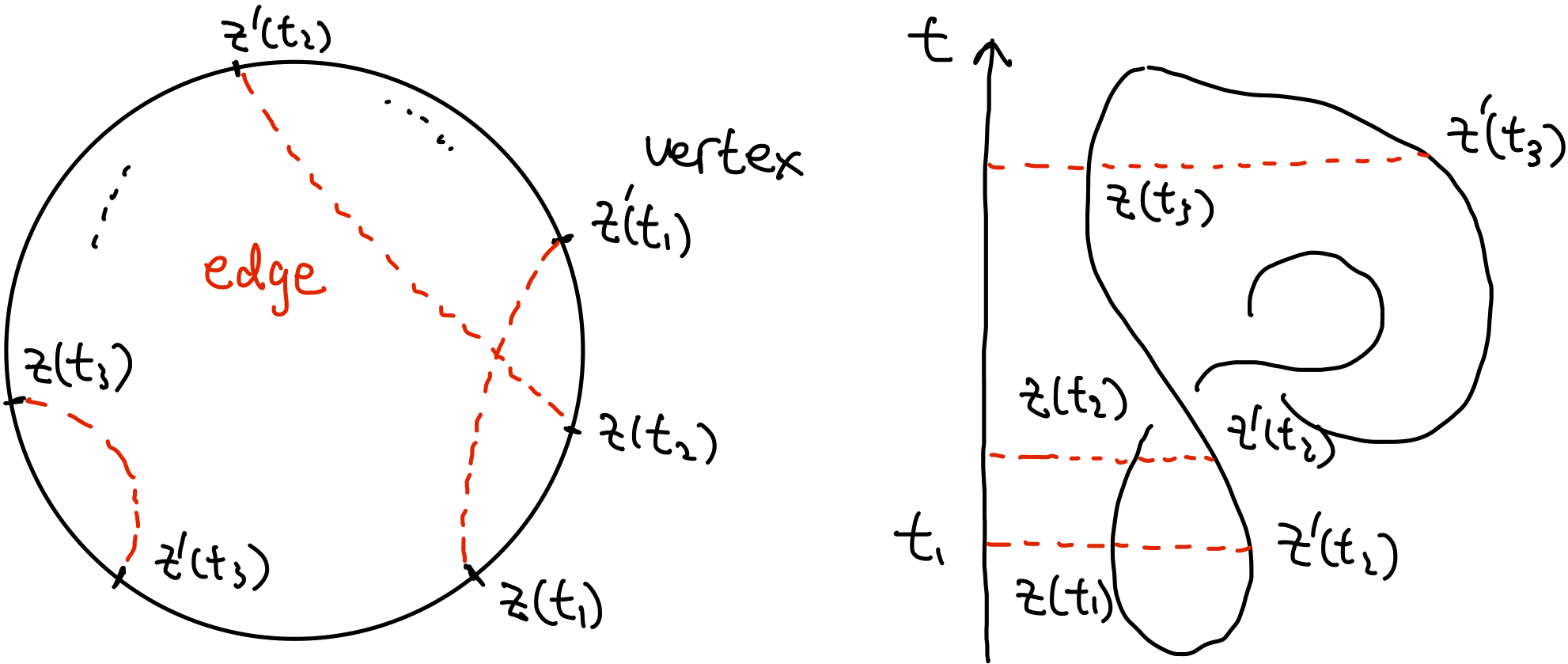
It is not hard to imagine that, since the Kontsevich integral is constructed from the perturbative expansion of Chern-Simons theory, it should be invariant under isotopy of the knot $𝐾$ .

However, such naive expectation is not true under an arbitrary isotopy of the knot $𝐾$ . For example, consider a isotopy which would create or annihilate a pair of critical points in the height function along the knot $𝐾$ , the Kontsevich integral would not be invariant under such isotopy.

If we restrict to isotopies that preserve the Morse nature of the knot $𝐾$ , the Kontsevich integral would be invariant under such isotopies.

Any deformation of a knot within the class of Morse knots can be approximated by a sequence of deformations of three types:

Orientation- preserving reparametrizations, which is trivial to verify the invariance of the Kontsevich integral.
Horizontal deformations: preserves all horizontal planes ${𝑡 = const}$ and leaves all the critical points (together with some small neighbourhoods) fixed.
Movements of critical points.

Now we focus on last two types of deformations.

Horizontal Deformations

The horizontal deformations could be viewed as an isotopy of a tangle which fixes the boundary points. Consider two tangles $𝑇_{0}$ and $𝑇_{1}$ , which are related by a horizontal deformation $𝑇_{𝜆}$ , $𝜆 \in [0, 1]$ .

The Kontsevich integral over $𝑇_{1}$ and $𝑇_{0}$ could be related with the integration over the boundary of the parameter space $Δ = Δ_{0} \times [0, 1]$ , where $Δ_{𝜆} ≔ {0 < 𝑡_{1} < \dots < 𝑡_{𝑛} < 1} \times {𝜆}$ is the standard $𝑛$ -simplex over $[0, 1]$ at fixed $𝜆$ . By Stokes theorem, we have:

\int_{𝜕 Δ} 𝜔 = \int_{Δ} 𝑑 𝜔 \overset{𝑑 𝜔 = 0}{⟶} 0,

where $𝜕 Δ = Δ_{1} - Δ_{0} + \dots$ , and $\dots$ denotes the contributions from the (codimension $1$ ) boundary strata characterized by some two points collapsing configuration, i.e.:

\int_{Δ_{1}} 𝜔 - \int_{Δ_{0}} 𝜔 + \int_{𝜕 Δ \times [0, 1]} 𝜔 = 0 .

Using the Fubini’s theorem, we only need to check the contributions from $𝜕 Δ$ to verify the invariance of the Kontsevich integral under horizontal deformations, i.e., we need to check that the contributions from $𝜕 Δ$ would vanish.

There are four types of such collapsing configurations:

Time plane hits a critical point.
Two chords end at two same points.
Two chords’ endpoints belong to four different strings.
Two chords’ endpoints belong to three different strings.

The first type of boundary strata would not contribute to the integral, since the integrand form would vanish at such boundary.

The second type of boundary strata would also not contribute to the integral, since the integrand form would vanish at such boundary due to the antisymmetry of the wedge product:

(𝑑 𝑧_{𝑘} - 𝑑 𝑧_{𝑘}^{'}) \land (𝑑 𝑧_{𝑘} - 𝑑 𝑧_{𝑘}^{'}) = 0,

while $𝑧_{𝑘} = 𝑧_{𝑘 + 1}$ and $𝑧_{𝑘}^{'} = 𝑧_{𝑘 + 1}^{'}$ .

The third type of boundary strata would not be naively zero. We denote the four different strings as $1, 2, 3, 4$ , and the two collapsing chords, for example $(1, 3)$ and $(2, 4)$ , denoted by their end-strings.

The possible collapsing configurations could be constructed by the following two ways:

$𝑘$ chord is $(1, 3)$ and $𝑘 + 1$ chord is $(2, 4)$ .
$𝑘$ chord is $(2, 4)$ and $𝑘 + 1$ chord is $(1, 3)$ .

And there are two additional chord connecting $(1, 2)$ and $(3, 4)$ respectively. Thus, the contributions from these two collapsing configurations could be expressed as:

(1, 2) \land (3, 4) \land \frac{𝑑 𝑧_{𝑘} - 𝑑 𝑧_{𝑘}^{'}}{𝑧_{𝑘} - 𝑧_{𝑘}^{'}} \land \frac{𝑑 𝑧_{𝑘 + 1} - 𝑑 𝑧_{𝑘 + 1}^{'}}{𝑧_{𝑘 + 1} - 𝑧_{𝑘 + 1}^{'}} + (1, 2) \land (3, 4) \land \frac{𝑑 𝑧_{𝑘 + 1} - 𝑑 𝑧_{𝑘 + 1}^{'}}{𝑧_{𝑘 + 1} - 𝑧_{𝑘 + 1}^{'}} \land \frac{𝑑 𝑧_{𝑘} - 𝑑 𝑧_{𝑘}^{'}}{𝑧_{𝑘} - 𝑧_{𝑘}^{'}} = 0,

(where $𝐷_{𝑝}$ for such configuration is same) thus, the third type of boundary strata would also not contribute to the integral.

The last type of boundary strata is the most interesting one. We could construct such collapsing configurations by the following $6$ ways by traversing all linking situations:

using the fact that $𝜔_{𝑖 𝑗} = 𝜔_{𝑗 𝑖}$ , the equation above is identified with Arnold’s identity:

𝜔_{12} \land 𝜔_{23} + 𝜔_{23} \land 𝜔_{13} + 𝜔_{13} \land 𝜔_{12} = 0,

thus, the last type of boundary strata would also not contribute to the integral. Therefore, we conclude that:

Theorem

the Kontsevich integral is invariant under horizontal deformations of the Morse knot

𝐾

Theorem

the Kontsevich integral is invariant under horizontal deformations of the Morse knot

𝐾

Movements of Critical Points

Kontsevich integral is not an invariant under movement of critical points. Under such deformation, the Kontsevich integral would change by ${Φ (\infty)}^{\frac{1}{2}}$ , which is the Kontsevich integral of the unknot (for further discussion, check this). Thus, the normalized Kontsevich integral defined as:

{\hat{Φ}}_{𝑛, 𝑐} (𝐾) = \frac{Φ_{𝑛} (𝐾)}{{(Φ (\infty))}^{\frac{𝑐}{2}}},

where $𝑐$ is the number of critical points of the Morse knot $𝐾$ . This normalization factor would cancel the framing anomaly in Chern-Simons theory as well. This is called the universal Vassiliev invariant.

Application: Quantum Yang-Baxter Equation

Yang-Baxter equation could be understood as the invariance of Kontsevich integrals under Reidemeister move of type III in knot theory. In the context of anyons, this could be interpreted as the consistency condition of braiding among three anyons.

Thus, the integration would be modeled by a $3$ -strands tangle, and the integration over the boundary of $Δ \times [0, 1]$ would leads to:

Φ_{𝑛} (𝑇_{1}) - Φ_{𝑛} (𝑇_{0}) + \int_{𝜕 Δ \times [0, 1]} 𝜔 = 0,

where $𝑇_{0}$ and $𝑇_{1}$ are two tangles related by Reidemeister move of type III.

This is exactly the same situation as the horizontal deformation case discussed above. Thus, using the same argument as before, the contributions from the boundary strata would vanish. What we left is $Φ_{𝑛} (𝑇_{1}) = Φ_{𝑛} (𝑇_{0})$ , which is the $ℏ^{𝑛}$ -th order (Quantum) Yang-Baxter equation.

¹This is the simplest case of the so-called connected diagram expansion in quantum field theory.
²Well, you may argue that there is a (slight) difference of a factor $ℎ^{\lor}$ in the definition of $ℏ$ at the case of CS and KZ respectively. However, since the perturbative expansion is done at large $𝑘$ limit (small $ℏ$ ), this difference could be ignored. Also, it is quite interesting to restore this factor $ℎ^{\lor}$ from the perturbative CS theory point of view, which I don’t know how to do so.

Back to all articles