Mixed Anomaly and Riemann-Roch Theorem

This blog is aim to explain how the mixed anomaly between $𝑈\left(1\right)$ symmetry and gravity in $𝑏𝑐$ CFT leads to the Riemann-Roch theorem in complex geometry. In this blog, we will just focus on the main physical idea, and leave the rigorous mathematical treatment to future posts.

Introduction: Monopole Inside a Sphere

Consider a monopole inside a sphere ${𝕊}^2$, there is no global well-defined gauge connection $𝐴$ over ${𝕊}^2$. One needs to use some patches $\left\{{𝑈}_{𝑖}\right\}$ to cover ${𝕊}^2$, then define ${𝐴}_{𝑖}\in {\mathrm{\Omega }}^1\left({𝑈}_{𝑖}\right)$ (after identify a reference connection), and using transition functions $\left\{{𝑓}_{𝑖𝑗}\right\}$ to obtain global $𝑈\left(1\right)$ connection.

For the situation of ${𝕊}^2$, the simplest choice of patches might be two hemispheres, where the intersection of two patches is a circle ${𝕊}^1$. Thus, one can easily prove that, the connection could be written as:

where the associated gauge curvature could be written as $𝐹=\frac{1}{2}d𝑆$, and the transition function could be written as ${\mathrm{e}}^{𝑖𝜑}:𝐴\mapsto 𝐴+d𝜑$. Using the formula above, the flux could be calculated by:

bc CFT and U(1) Current

Local Description

Consider the $𝑏𝑐$ CFT over a Riemann surface $𝑋$ with conformal weight $\left(𝜆,0\right)$ and $\left(1-𝜆,0\right)$:

where $𝑏\in \mathrm{\Gamma }\left(𝑋,{𝐿}^{\otimes 𝜆}\right)$, $𝑐\in \mathrm{\Gamma }\left(𝑋,𝐾\otimes {𝐿}^{-\otimes 𝜆}\right)$, $𝐿$ is a holomorphic line bundle and $𝐾$ is the canonical bundle over $𝑋$.

Now we consider the local description of this CFT over a patch $𝑈\approx ℂ$ with local coordinate $𝑧$. The energy-momentum tensor under this coordinate is given by:

and the $𝑈\left(1\right)$ current is:

The OPE for the current could be written as:

which implies the current changing while one consider the conformal transformation $𝑧\mapsto 𝑤$:

The last equality holds because the conformal translation is holomorphic. This translation formula implies that $𝐽\left(𝑤\right)$ is not a primary field.

The conserved quantity here from classical mechanics could be naively written as ${\int }_{\mathrm{\Sigma }}𝜕𝐽d𝑥=0$. This equation is true on $ℂ$ with compact supported $𝑏𝑐$ fields. However, more precisely consideration is needed while we consider the global structre of this field theory.

Glue Patches from Local Data

While we want to glue patches into one dimensional complex manifold, a holomorphic function $𝑓$ satisfies ${𝜕}_{𝑧}𝑓\left(𝑝\right)\ne 0$ would play a role as transition function, which indeed is a conformal transformation $𝑧\mapsto 𝑤$. Thus, recall the discussion in the intro, the integration of $𝜕𝐽$ over $𝑋$ should be rephrased as the integration over multiple patches glued by some conformal transformation:

Here we chose a good over ${𝑈}_{𝑖}$ of $𝑋$ and attach local coordinates $\left\{{𝑧}_{𝑖}\right\}$ on each patch. Since $𝐽\left({𝑧}_{𝑖}\right)$ is $\left(1,0\right)$ form over ${𝑈}_{𝑖}$, the integration above could be rewritten as:

Given a (good) cover $\mathrm{𝒰︀}≔\left\{{𝑈}_{𝑖}\right\}$ of $𝑋$, transition function is given by ${𝑓}_{𝑖𝑗}:{𝑧}_{𝑗}\mapsto {𝑓}_{𝑖𝑗}\left({𝑧}_{𝑖}\right)$, thus the current on two patches are related by:

For now, we have met a similar situation as the monopole inside a sphere, where the current $𝐽$ plays the role of gauge connection $𝐴$ which might not be globally well-defined.

A way to formulate the consideration in the intro, where we first integrate $d𝐽$ over each patch, then sum them up with the transition function.

One can embed the consideration above into Čech complex, where $𝐽\left({𝑧}_{𝑖}\right)$ is an element in ${𝐶}^0\left(\mathrm{𝒰︀},{\mathrm{\Omega }}^1\right)$, and $\frac{1-2𝜆}{2}d\left(ln{𝜕}_{{𝑧}_{𝑖}}{𝑓}_{𝑖𝑗}\right)$ is an element in ${𝐶}^1\left(\mathrm{𝒰︀},{\mathrm{\Omega }}^1\right)$, where:

• The first cohomology degree in ${𝐶}^{•}$ is the intersection number of patches, e.g., ${𝑈}_{𝑖}$ is an element in ${𝐶}^0$, ${𝑈}_{𝑖}\cap {𝑈}_{𝑗}$ is an element in ${𝐶}^1$ and so on.
• The second cohomology degree in ${\mathrm{\Omega }}^{•}$ denotes the degree of differential forms, e.g., ${\mathrm{\Omega }}^0$ is degree $0$ form (function), ${\mathrm{\Omega }}^1$ is degree $1$ form and so on ¹.

And the associated Čech differential is induced by:

• $𝛿:{𝐶}^{𝑝}\left(\mathrm{𝒰︀},{\mathrm{\Omega }}^{𝑞}\right)\mapsto {𝐶}^{𝑝+1}\left(\mathrm{𝒰︀},{\mathrm{\Omega }}^{𝑞}\right)$, where $𝛿:{𝑓}_{{𝑖}_1,\dots ,{𝑖}_{𝑛}}\mapsto {\left(𝛿𝑓\right)}_{{𝑖}_1,\dots ,{𝑖}_{𝑛},{𝑖}_{𝑛+1}}$.
• $d:{𝐶}^{𝑝}\left(\mathrm{𝒰︀},{\mathrm{\Omega }}^{𝑞}\right)\to {𝐶}^{𝑝}\left(\mathrm{𝒰︀},{\mathrm{\Omega }}^{𝑞+1}\right)$ is the standard de Rham differential over a patch ${𝑈}_{{𝑖}_1,\dots ,{𝑖}_{𝑛}}$.

Therefore, the transition of current $𝐽$ could be rephrased as:

which could be rewritten as:

where the arrow $𝑎\stackrel{𝛿}{\to }𝑏$ denotes $𝑏=𝛿𝑎$. Moreover, since transition functions satisfying the condition

we have:

where $d$ would act as an embedding ${𝐻}^2\left(𝑋,\mathbb{Z}\right)\hookrightarrow ︎{\mathrm{\Omega }}^0\left({𝑈}_{𝑖𝑗𝑘}\right)$ i.e., $d:𝑛\mapsto {𝑛}_{𝑖𝑗𝑘}$ for $\left[𝑛\right]\in {𝐻}^2\left(𝑋,\mathbb{Z}\right)$. Note that our integration is over $𝑋$ for $𝜕𝐽$, then we need to include $𝜕𝐽=d𝐽$ into the consideration, thus we have:

where $𝛿$ is the restriction of a smooth form to the intersection of patches, i.e. $𝛿:𝜔\mapsto 𝜔{|}_{{𝑈}_{𝑖}}$, for $𝜔\in {\mathrm{\Omega }}^2\left(𝑋\right)$.

Using the diagram above, we could replace the ill-defined integration of $𝜕𝐽$ over $𝑋$ by the well-defined integration of $d{𝐽}_{𝑖}$ over each patch ${𝑈}_{𝑖}$, then by the globally well-defined $2$-form $𝜔\in {\mathrm{\Omega }}^2\left(𝑋\right)$.

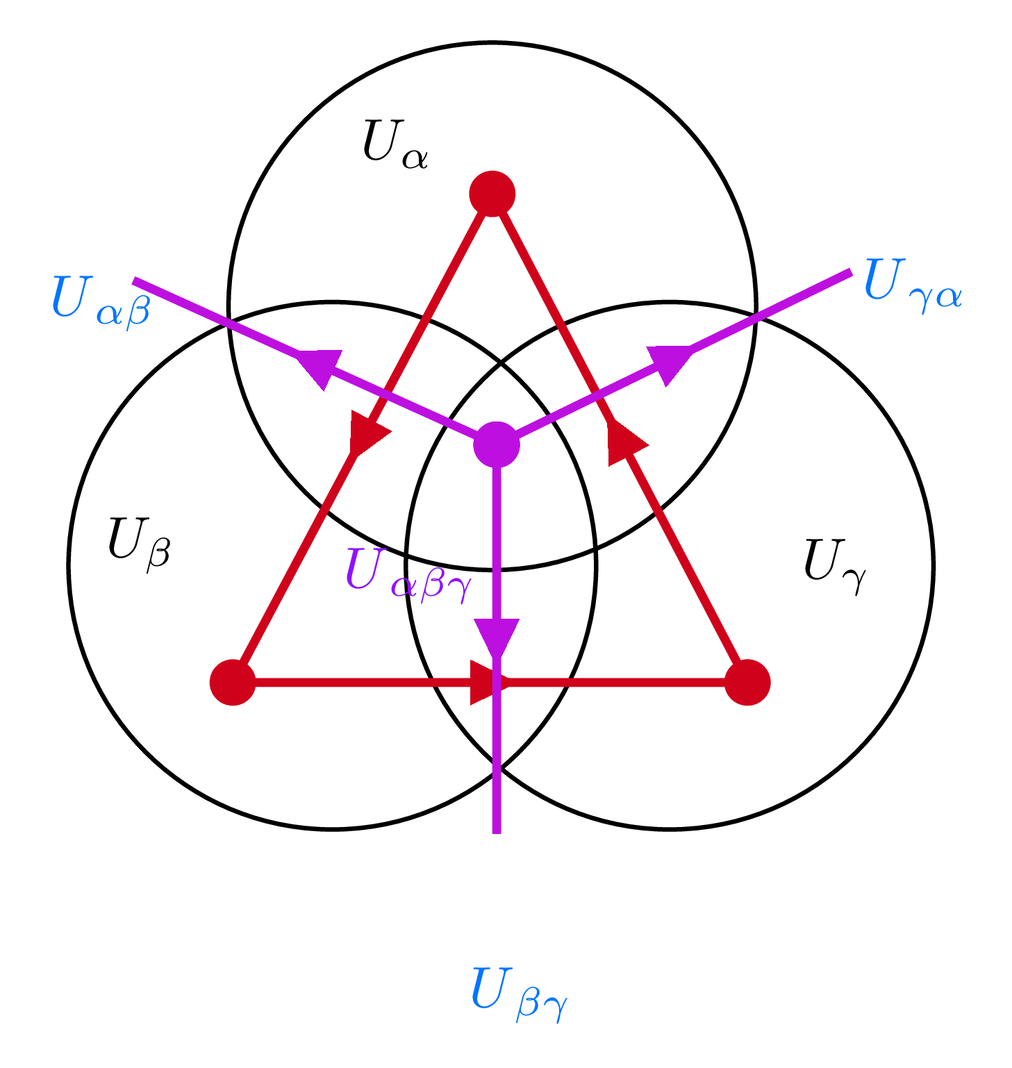
Moreover, the diagram above hints that, the integration of $𝜔$ over $𝑋$ would descend to the sum of $\left(1-2𝜆\right)𝑖𝜋{𝑛}_{𝑖𝑗𝑘}$ over all ${𝑈}_{𝑖𝑗𝑘}$. To see this, we consider the nerve of cover $\mathrm{𝒰︀}$, which is a simplicial complex constructed from $\mathrm{𝒰︀}$. See the figure below for an example of nerve of cover (and its dual).

Thus, the integration of $𝜔$ over $𝑋$ could:

• First, be rephrased as the integration over the boundary ${𝑒}_{𝑖𝑗}$:

where ${𝑒}_{𝑖𝑗}$ denotes the edge correspond to the intersection ${𝑈}_{𝑖}\cap {𝑈}_{𝑗}$,

• Then, be rephrased as the integration over the face ${𝑓}_{𝑖𝑗𝑘}$, which is simply the sum of ${𝑛}_{𝑖𝑗𝑘}$:

where ${𝑓}_{𝑖𝑗𝑘}$ denotes the face correspond to the intersection ${𝑈}_{𝑖}\cap {𝑈}_{𝑗}\cap {𝑈}_{𝑘}$.

• Finally, be rephrased as the ‘integration’ of $𝑛$ over $𝑋$, i.e., the pairing of $\left[𝑛\right]\in {𝐻}^2\left(𝑋,\mathbb{Z}\right)$ with the fundamental class $\left[𝑋\right]\in {𝐻}_2\left(𝑋,\mathbb{Z}\right)$:

which is precisely the first Chern class ${𝑐}_1\left(𝐿\right)\in {𝐻}^2\left(𝑋,\mathbb{Z}\right)$ of line bundle $𝐿$ by definition, multiplied by $\left(1-2𝜆\right)𝑖𝜋$.

Therefore, the integral of $𝜕𝐽$ (in fact, $𝜔$) over Riemann surface $𝑋$ gives

where ${𝑐}_1\left(𝐿\right)\in {𝐻}^2\left(𝑋,\mathbb{Z}\right)$ is the first Chern class of line bundle $𝐿$.

Zero Modes, Riemann-Roch and Index

Zero Modes and Index

The zero mode equation for $𝑏𝑐$ CFT could be written as:

We denote the number of zero modes for $𝑏$, $𝑐$ fields as $𝐵$ and $𝐶$ respectively. It is easy to identify that $𝐶=ker\left({𝜕}_{𝐾\otimes {𝐿}^{-𝜆}}\right)$ and $𝐵=ker\left({𝜕}_{{𝐿}^{𝜆}}\right)$, thus the difference of the zero modes is given by:

using Serre duality ${𝐻}^{𝑖}\left(𝑋,\mathrm{𝒪︀}\left(𝐾\otimes {𝐿}^{-𝜆}\right)\right)\approx {𝐻}^{𝑛-𝑖}{\left(𝑋,\mathrm{𝒪︀}\left({𝐿}^{𝜆}\right)\right)}^{\vee }$, one have (in our case, $𝑛=1$):

thus the index of elliptic operator $𝜕$ could be rephrased as:

Moreover, it is well-known that the difference of zero modes could be rephrased as the charge of $𝑈\left(1\right)$ Noether current, which is given by the $𝑈\left(1\right)$ generator (at quantum level):

We can use the path integral to evaluate this charge, which we have:

where $𝑑𝜇$ is a formal Berezin measure over the space of fields, and $𝑍$ is the partition function.

Note that the possible zero modes of $𝑏𝑐$ fields would never shown in the action $𝑆\left[𝑏,𝑐\right]$, thus the integration above would always vanish unless there is no zero modes. To overcome this problem, one need to insert an observable with $𝐵$ $𝑏$ fields and $𝐶$ $𝑐$ fields into the integration, i.e.:

we will finally show shat this integration is independent of the choice of $\mathrm{𝒪︀}$, but now let me choose a simple form of this operator:

thus, the $𝑈\left(1\right)$ charge operator would acts on this observable as:

which could be derived from

and Leibniz rule of commutator.

Now we consider the path integral version of the commutator above. In order to realize such commutator above, we need two facts above:

• First, the path integral would lead to a (time, radial) ordered product.
• Second, the quantity of $𝑄$ is robust under a small deformation of integral path (using Cauchy’s integral formula).

The first fact shows that we could realize the quantum expectation value as:

Using the second fact, these two loops could be deformed as a closed loop around $𝑂\left(𝑧\right)$. Thus, the commutator could be realized simply as the path integral expectation value of $𝑄𝑂$.

Using the result above for each $𝑏\left({𝑧}_{𝑖}\right)$ and $𝑐\left({𝑤}_{𝑗}\right)$, we finally obtain:

which is independent of the choice of $\mathrm{𝒪︀}$. Thus, we have identified the index of elliptic operator $𝜕$ with the $𝑈\left(1\right)$ charge:

Mixed Anomaly and Riemann-Roch Theorem

Recalling our previous result, this actually gives the relationship between ghost number and manifold Euler characteristic:

here we used the fact that $𝜒\left({𝐿}^{𝜆}\right)=deg\left({𝐿}^{𝜆}\right)=𝜆deg\left(𝐿\right)$ and $deg\left(𝐿\right)=2-2𝑔$, where $𝐿$ is the canonical line bundle over $𝑋$. Noting the equivalence between ghost number and index, we finally obtain the index theorem for elliptic operator $𝜕$:

Using the index expression $\text{ind}\left(𝜕\right)={ℎ}^0\left(𝑋,\mathrm{𝒪︀}\left({𝐿}^{𝜆}\right)\right)-{ℎ}^1\left(𝑋,\mathrm{𝒪︀}\left({𝐿}^{𝜆}\right)\right)$, this is precisely the Riemann-Roch theorem:

Using the line bundle-divisor correspondence, this theorem can be transformed into the standard form found in textbooks.

1. ¹$\left(1,0\right)$ form over ${𝑈}_{𝑖}$ could be naturally embedded into ${𝐶}^0\left(\mathrm{𝒰︀},{\mathrm{\Omega }}^1\right)$, so that we write $𝐽\in {𝐶}^0\left(\mathrm{𝒰︀},{\mathrm{\Omega }}^1\right)$.